Deep Learning in Medical Imaging
Article information

Abstract
The artificial neural network (ANN), one of the machine learning (ML) algorithms, inspired by the human brain system, was developed by connecting layers with artificial neurons. However, due to the low computing power and insufficient learnable data, ANN has suffered from overfitting and vanishing gradient problems for training deep networks. The advancement of computing power with graphics processing units and the availability of large data acquisition, deep neural network outperforms human or other ML capabilities in computer vision and speech recognition tasks. These potentials are recently applied to healthcare problems, including computer-aided detection/diagnosis, disease prediction, image segmentation, image generation, etc. In this review article, we will explain the history, development, and applications in medical imaging
INTRODUCTION
Artificial intelligence (AI) technology, powered by advanced computing power, a large amount of data, and new algorithms, becomes more and more popular. It has been applied to various kinds of fields such as healthcare, manufacturing and convenient living life, so on. AI, in general, has 3 categories. One is a symbolic approach that outputs answers using a rule-based search engine. Another is the Bayesian theorem-based approach. The other is the connectionism approach based on deep neural networks (DNNs). While each approach has its strengths and weaknesses, the connectionism approach is recently gaining a lot of attention to solve complex problems.
Machine learning (ML) is a subset of AI that learns data itself with minimum human intervention to classify categories or predict future or uncertain conditions [1]. Since ML is data-driven learning, it is categorized into nonsymbolic AI and can predict from unseen data. Here, ML tasks include regression, classification, detection, segmentation, etc. Generally, data sets of ML consist of exclusive training, validation, and test sets. It learns characteristics of data from the training data set and validates the learned characteristics from the validation data set. Finally, one can confirm the accuracy of ML by using the test data set.
As a part of ML, an artificial neural network (ANN) is a brain-inspired algorithm that consists of layers with connected nodes. It consists of input and output layers with hidden layers. Here, the first layer has input values and the last layer has corresponding labeled values. During training, the value of each node is determined by parameterizing weights through learning algorithms such as back propagation. Weights for each node are optimized towards the direction to reduce losses and thus increase accuracy. By iterating the backpropagation, optimized weights can be obtained. However, ANN has limitations that sometimes the training ends up in a local minimum or optimized only for trained data which results in overfitting problems. Recently researchers progress a deep learning to expand ANN into DNN by stacking multi-hidden layers with connected nodes between input and output layers. The multilayer can deal with more complex problems by composing simple decisions between layers. DNN generally shows better performance than the shallow layered network in prediction tasks such as classification and regression [2]. Each layer of DNN optimized its weights based on the unsupervised restricted Boltzmann machine [3] to prevent learning converges at local minimum or overcome overfitting problems. Recently, residual neural networks is also known to avoid vanishing gradient problem using skip connections [2]. Besides, the advent of big data and graphics processing units could solve complex problems and shorten the computation time.
Accordingly, the deep learning algorithm gets a lot of attention these days to solve various problems in medical imaging fields. One example is to detect disease or abnormalities from X-ray images and classify them into several disease types or severities in radiology [4,5]. This kind of task has been executed based on the various ML algorithms with proper optimization, theoretical or empirical approaches. One example is computer-aided detection (CAD) systems which were developed and applied to the clinical system since the 1980s. However, the CAD system generates more false positives than physicians and thus led to the increment of assessment time and unnecessary biopsies [6,7]. Thanks to the deep learning technology, these problems could have been overcome with great answering accuracy and allow humans to spend time on other productive tasks. However, the advent of this technology does not mean the ultimate replacement of physicians, especially radiologists. Instead, it helps radiologists to diagnose patients more accurately.
1. Supervised and Unsupervised Learning
Primary ML methods are categorized into supervised learning, unsupervised learning and reinforcement learning (RL). RL is not adequate to medical application, because the decision of a RL system affects both the patient’s future health and future treatment options. As a result, long-term effects are harder to estimate [8]. The main difference between supervised and unsupervised learnings is whether the training data set has labeled outputs corresponding to input data. The supervised learning infers a mathematical relationship between the inputs and the labeled outputs while the unsupervised learning infers a function that expresses hidden characteristics reside in input data. In supervised learning, output data can have categorical value or numerical continuous value depending on its task. It becomes a classification or a pattern recognition problem when the output data is in categorical value while it becomes a regression problem when the output data is in continuous numerical value. Here, the classification task can be binary, multiclass or multilabeled where the multilabeled means more than one class exists in each input data. On the other hand, unsupervised learning includes cluster analysis, principal component analysis, and generative adversarial networks (GANs). In addition, semisupervised learning is also widely used when one has a small amount of labeled data set. Since acquiring the labeled data is generally very difficult or very expensive, semisupervised learning could be cost-effective.
In supervised learning, K-nearest neighbors (KNN) is the simplest ML algorithm for classification or regression tasks [9]. It finds K numbers of nearest data points from input data and votes to decide its class in a classification task. In a regression task, a value of input point is decided by averaging out K numbers of nearest data points. However, prediction through KNN gets slower when the number of training data becomes higher [10]. On the other hand, linear regression eliminates this problem [11]. Linear regression parameterizes a linear model with given training data. Once the parameter of a linear model is optimized, the prediction of a given data is just an output from the best-fit formula. Support vector regression and ANN are widely used nowadays since they show better performances in various regression problems [12]. Similarly, logistic regression, random forest and support vector machine are widely used for classification [13]. Logistic regression parameterizes the logistic model to predict binary classification. Recently, ensemble learning, by combining various classification algorithms for more accurate prediction, is commonly used [14].
2. Convolutional Neural Network
As a part of deep learning, a convolutional neural network (CNN) is recently spotlighted in computer vision for both supervised and unsupervised learning tasks [15]. The CNN has broken the all-time records from traditional vision tasks [16]. The compositions of CNN are convolutional, pooling and fully connected layers. The primary role of the convolutional layer is to identify patterns, lines, and edges so on. Each hidden layer of CNN consists of convolutional layers that convolve input array with weight-parameterized convolution kernels. The multiple kernels generate multiple feature images and made succeed in various vision tasks such as segmentation and classification. Between the convolutional layers, feature maps are locally progressively and spatially pooled pooling layers. The pooling layer transfers the maximum or average value and thus reduces the size of feature maps. This process catches features of an image with robust to the position and shape. Empirically, max pooling process is generally used. The CNN architecture is composed of alternating these convolutional and pooling layers repeatedly. For the classification or regression tasks, the fully connected layers are attached at the end of the CNN architecture and provide a final decision. During training, a loss is estimated by differencing labeled value and predicted value. On the other hand, in the segmentation task, convolutional layers and up-sampling layers are attached at the end of pooling layers to reconstruct the size of the input image. Thus, training loss is evaluated by differencing labeled mask image and reconstructed output image through CNN. Since CNN architecture is composed of many layers, a number of parameters for training can reach millions. This means a lot of data is needed for training needs to acquire competent accuracy. The number of data depends on task purpose and image characteristics. For instance, at least 1,000 images per class are necessary to get a competent result in a classification task if one trains the data from scratch. However, data collection is usually very difficult and even more hard if one also needs labeled data. To overcome this problem, data augmentation is also tried in general task which generates images from a limited number of data using image transformation methods such as rotation, translation, scaling, flipping, so on [17].
RADIOLOGICAL APPLICATIONS
In this chapter, various kinds of radiologic applications in classification, object detection, image segmentation, image generation, and image transformation were discussed.
1. Image Classification
One key task for radiologists is an appropriate differential diagnosis for each patient’s medical images, and this classification task includes a wide range of applications from determining the presence or absence of a disease to identifying the type of malignancy. Recently introduced DNN, especially CNN, has improved imaging-based classification performance in various medical applications, including the diagnosis of tuberculosis, diabetic retinopathy, and skin cancers [18-20]. Since medical images contain various sizes and types of complex disease patterns, it would be difficult for the CNN models to directly train complicated disease patterns. These complex problems could be solved by curriculum learning strategy that involves gradual training of more complex concepts [21]. This curriculum learning with weak labeling of high-scale chest X-ray scans performed well for classification of 5 disease patterns and required less preparation to train the model [22]. Deep learning requires a large amount of data to minimize overfitting and improve the performances, whereas it is difficult to achieve these big datasets with medical images of low-incidence serious diseases in general practice. Thus, a better classification strategy is needed for these small datasets. Combination of radiomic features and multilayer perceptron network classifier served a high-performing and generalizable model for a small dataset with heterogeneous magnetic resonance imaging (MRI) protocols [23]. Furthermore, CNNs could be incorporated into current radiomics model by extracting a large number of deep features from hidden layers of it [24,25]. These deep features which are evaluated not by feature engineering (handcrafted) but by feature learning could contain more abstract information of medical images and provide more predictive patterns compared with the handcrafted features.
2. Object Detection
Object detection is finding and categorizing objects. In biomedical images, a detection technique is also performed to identify the areas where the patient’s lesions are located as box coordinates. Deep learning-based object detection can be composed of 2 types. One is the region proposal-based algorithms [26-28]. This approach extracts various types of patches using a selective search algorithm from input images. Afterward, the trained model decides whether multiple objects exist in each patch and classifies objects based on region of interest (ROI). Specifically, the region proposal network was developed to increase the speed of the detection process [28]. The other techniques performed the object detection using the regression method as one stage network [29-32]. These approaches are directly finding and detecting bounding box coordinates and class probabilities from image pixels in whole images [29-31]. Although the region proposal approach as 2-stage network shows better performance in terms of accuracy, the regression-based model as one stage network is better in terms of speed as well as accuracy. Recently, RetinaNet [32] has been introduced to complement the disadvantage of 1 stage network. This network has applied focal loss [32] to solve the problem caused by extreme foreground-background data or class imbalance. Various object detection algorithms proposed for biomedical images are based on strong labels of per-pixel or the coordinated of bounding box coordinates. To acquire strong labels for detecting disease patterns or conditions is expensive and inevitable in medical environments. To overcome the cost of annotation data, we should exploit a transfer learning with the pretrained weight of the model learned from general natural images or a large number of medical images like national institutes of health dataset and fine-tune the model with a small number of medical images.
For example, we introduce deep learning techniques through a spine sagittal X-ray. The spine sagittal X-ray plays an important role in clinical diagnosis and operation plans in spine patients. We developed deep learning algorithms to acquire sagittal parameter data of the whole spine X-ray. The training procedure to detect the parameter of the sagittal X-ray consists of 2 steps in Fig. 1. First, the regional patterns of spine X-ray images were identified by RetinaNet with spine X-ray images. Second, the coordinates of x and y as landmarks to diagnose spine patients were inferred by U-Net with the detected ROI images. Table 1 shows the error of landmark prediction. Fig. 2 shows the results of the detection of ROI images in the spine sagittal X-ray using RetinaNet. Fig. 3 shows the results of point detection in the spine sagittal X-ray with RetinaNet and U-Net. Each is the best, mean, and worst results. Fig. 4 shows the results of point detection in spine sagittal X-ray with RetinaNet and U-Net. Each result is the best, mean, and worst results. All results are totally able to detect and find point information to diagnose patients in spine sagittal X-ray.
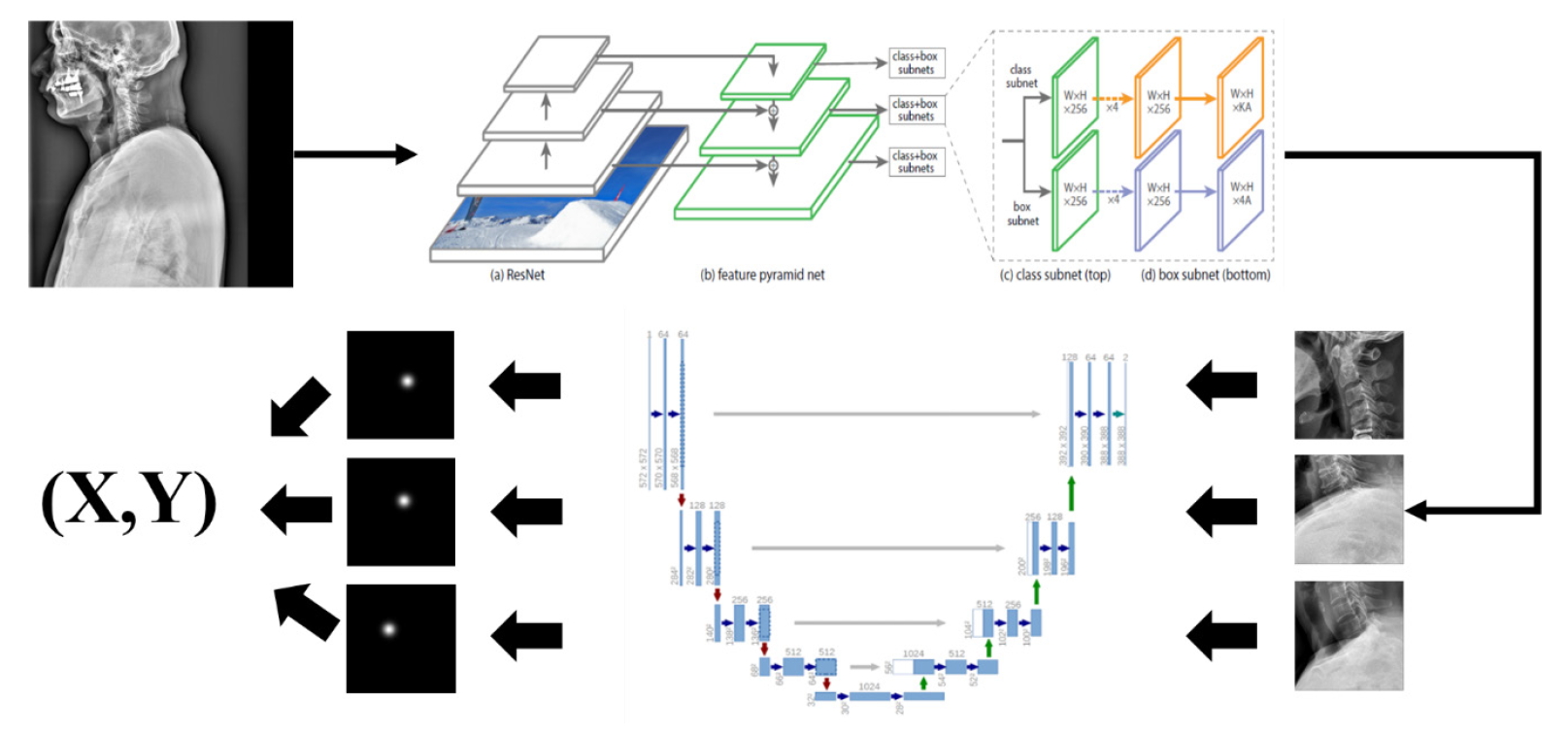
Network for detecting landmarks to plan spine surgery of patients in spine sagittal X-ray. From the detection of region of interest in images, landmarks were segmented with U-Net, and its corresponding coordinates (x and y) were evaluated.
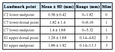
The error of landmark prediction based on cascaded convolutional neural net
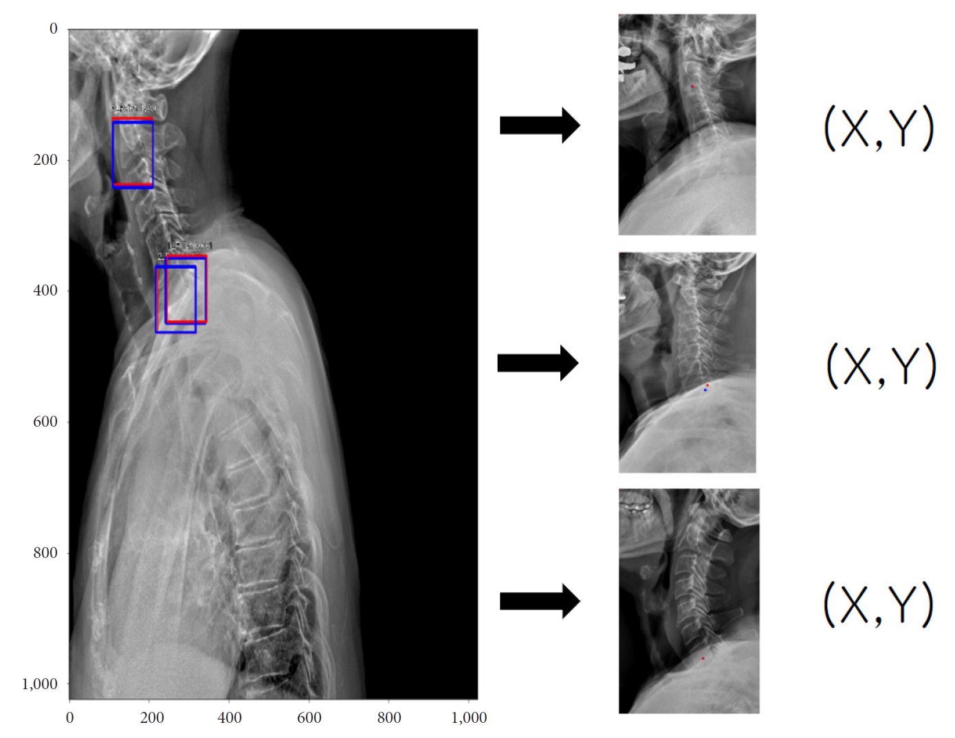
A typical example for detecting of region of interest (ROI) images (left; red, gold standard; blue, prediction ROI) and their coordinates (x and y) of corresponding landmarks in spine sagittal X-ray.
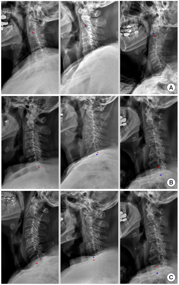
Examples of landmark detections of c-spine region in spine sagittal X-ray (best case in left column, mean case in middle column, and the worst case in right column; red, gold standard; blue, prediction). (A) Landmark of C2 lower midpoint, (B) landmark of C7 lower dorsal point, and (C) landmark of C7 lower midpoint.
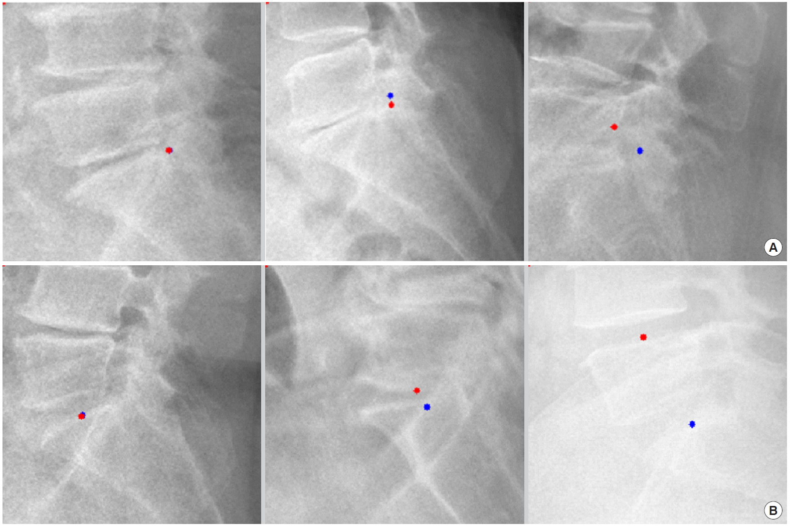
Examples of landmark detections of l-spine region in spine sagittal X-ray (best case in left column, mean case in middle column, and the worst case in right column; red, gold standard; blue, prediction). (A) Landmark of S1 upper dorsal point and (B) landmark of S1 upper midpoint.
3. Image Segmentation and Registration
As medical images provide a lot of information, various automatic segmentation and registration algorithms have been studied and proposed for use in clinical settings. In recent years, deep learning technology has been used for analysing medical images in various fields, and it shows excellent performance in various applications such as segmentation and registration.
The classical method of image segmentation is based on edge detection filters and several mathematical algorithms. Using several techniques to improve targeted segmentation performance such as dependent thresholding and close-contour methods [33]. Alternatively, registration was attempted for segmentation [34]. To improve segmentation performance associated with medical images, DNNs, especially CNNs, have been gradually introduced. Attempts have been made for the segmentation of the tumors and other structures in the brain, lungs, biological cells, and membranes [35-37]. These approaches used patch-based 2-dimensional CNN techniques and postprocessing in the same way as classical ML. However, training a patch-based method can take a long time, and depending on the number of patches, learning might not be possible.
Several CNN architectures have been proposed that feed through entire images with better image resolution [37-39]. Long et al. [40] introduced the fully CNN (fCNN) for the segmentation of images, however, fCNNs produce segmentations of lower resolution as compared to input images. That was due to the successive use of convolutional and pooling layers, both of which reduce the dimensionality. To predict segmentation of the same resolution as the input images, Brosch et al. [38,39] proposed the use of a 3-layer convolutional encoder network for multiple sclerosis lesion segmentation. The combination of convolutional and deconvolutional layers allows the network to produce segments that are of the same resolution as the input images. Ronneberger et al. [41] was suggested novel architecture named U-NET using convolutional and deconvolutional layers with skip connections which enables to obtain highly accurate segmentation probability maps in fully convolutional layers.
As 2-dimensional segmentation performance increases well enough, research has been conducted to segment the multiple slices of MRI and computed tomography (CT). The 2.5-dimensional (2.5D) approaches were inspired that 2.5D has richer spatial information of neighboring pixels with less computational costs than 3-dimensional (3D) [42,43]. Yet, there were still limitations using 2D kernels, not applying 3D filters which can extract abundant volumetric information. The 3D extended U-Net model is developed to segment kidney [44]. The suggested model demonstrated 0.863 averaged intersection over union of a kidney from 3D volume. However, 3D U-Net has the disadvantage of not being able to put the whole image due to memory limitations and reducing the image input. To optimize this, there has been a lot of researches focusing on performance optimization while reducing computation [45-47].
Recently, deep learning networks for improving segmentation performance in medical imaging have been continuously proposed. Performing multitasks with segmentation and classification, regression or registration has synergy to gain more precise segmentation performance [48,49]. As segmentation performance increases, studies have been conducted to consider the uncertainty of labels [50]. Furthermore, due to the high cost of medical labels, Semisupervised/unsupervised learning approaches were suggested using unlabelled data [51-53]. Since these studies have not yet surpassed the segmentation performance of supervised learning, it is considered future value as a technology that can overcome the severe imbalances in medical imaging.
4. Image Generation
While many applications using CNN were introduced in medical imaging, it is often challenging to obtain high quality, balanced datasets with labels in the medical domain [54]. Medical images are mostly imbalanced, and time-consuming to obtain their labels. In addition, medical images are hard to obtain due to their privacy issues [55]. To overcome the issues, several studies exploit GAN to make realistic synthetic images of whole X-ray or CT or ROIs of specific lesions, such as liver cancer [56,57].
GAN is a combination of 2 different neural networks that can generate realistic synthetic images [58]. Since GAN was introduced in 2014, many applications using GANs were introduced in medical imaging. In many studies, GANs were primarily used to generate various imaging modalities such as X-ray, CT, magnetic resonance, positron emission tomography, histopathology images, retinal images, and surgical videos [56-71]. Generated images in the studies were mainly used for data augmentation to have a more balanced dataset for training neural networks of classification or segmentation. With the synthetic images, classification or segmentation accuracies were significant increases than those with the imbalanced dataset [72].
Another interesting application using GAN is anomaly detection in medical imaging. To generate realistic synthetic images, the model is trying to mimic the distribution of source images in the latent space during the training. If the model learned distribution of normal images (i.e., images without disease), one may use the model as a tool in anomaly detection. By exploiting the DCGAN (deep convolutional generative adversarial network) model [73], Schlegl et al. [74] introduced an unsupervised anomaly detection method to find a guide marker in OCT images. The method showed a high performance in marker detection (area under the curve=0.89) but the iteration process was timeconsuming. It was further improved for real-time anomaly detection in their recent study by adopting the encoder-decoder scheme in the model architecture [75]. The studies demonstrated potential of GANs in unsupervised anomaly detection in medical imaging.
5. Image Transformation
History of image to image translation goes back to Hertzmann et al. [76] In this study, a nonparametric model was developed for texture analysis. However, more recent studies focus on using CNN. These studies can be classified into 2 categories including studies with or without GAN.
IMAGE TO IMAGE TRANSLATION WITHOUT USING GENERATIVE ADVERSARIAL NETWORK
Rise of an image to image translation cannot be separated from style transfer. Gatys et al. [77] used CNN for artistic style transfer. Gu et al. [78] changed loss and reshuffled feature vectors to transfer style. They argue that feature reshuffling can be a complementary solution for parametric and nonparametric neural network style transfer. Though their success of transferring style, overabstraction of features made these algorithms unrealistic. To overcome this hurdle, Li et al. [79] used wavelet transformation as well as multilevel stylization. Following this research, Yoo et al. [80] devised the wavelet pooling layer to enable photorealistic style transfer.
CNN can be used in image denoising. Jain and Seung [81] show frontiers of denoising technique using CNN architecture. They compared the performance of the Markov random field method to that of CNN and showed the CNN network can be used in denoising. Not only CNN but also autoencoder (AE) can be used in denoising. Vincent et al. [82] developed denoising AE, and they also developed stacked denoising AE as well [83]. Batson and Royer [84] used the concept of J-invariant and designed the Noise-2Self concept. Interestingly, this is a single image-level denoising concept. Modality transfer can be also performed with the CNN network. Han [85] used an encoder-decoder network for MRI to CT to transfer modality.
1. Image to Image Translation With Using GAN
Isola et al. [86] used conditional GAN to perform image to image translation with pixel to pixel correspondence. This model is called a pix2pix network. To overcome the limitation that requires pixel to pixel correspondence, Zhu et al. [87] designed CycleGAN architecture which does not require pixel to pixel correspondence. Though CycleGAN can be applied to unmatched images, style transfer between more than 3 domains requires too many generators – about half of square of the number of domains. Choi et al. [88] solved this issue with one general generator and named this architecture as StarGAN. Chen et al. [89] used GAN to denoising pipeline. They used GAN to estimate noise distribution, and another CNN architecture subtracts estimated noise distribution from the original image. Kudo et al. [90] chose conditional GAN to make thicker CT to thinner CT. They used a 3-dimensional patch to make CT slice thinner. Wolterink et al. [91] borrowed concept of CycleGAN to generate CT from MRI. In short, similar image to image tasks can be performed with or without using GAN. However, there are no consensus or proven facts that which one shows more satisfactory results between using or without using GAN.
DISCUSSION AND CONCLUSIONS
From the ANN inspired by the human neuronal synapse system in the 1950s to deep learning technology, AI suggests its potential to perform better than humans in some visual and auditory recognition tasks, which may indicate its applications in medicine and healthcare, especially in medical imaging. There could be many kinds of applications of deep learning technology in medical imaging to enhance the burden of medical doctors, quality of healthcare system and patient outcomes. Besides, these kinds of intelligent technology could be applied to precision medicine, which involves the prevention and treatment strategies that consider individual variability [92]. The success of precision medicine is largely dependent on robust quantitative imaging biomarkers, which can be accomplished by deep learning. In particular, imaging is noninvasively and routinely performed for clinical practice and can be used to compute quantitative imaging biomarkers. Many radiomics studies have correlated imaging biomarkers with genomic expression or clinical outcome [93].
Even with many promising results from previous studies, there are several issues to be resolved before the introduction of deep learning in medical imaging as follows: Firstly, the high dependency on the quality and amount of training dataset, and the tendency of overfitting and bias should be considered. Considering the differences in disease prevalence, imaging modality and protocols in clinical settings across the world, a generalization of deep learning methods should be declared. The evaluation methods to test the performance of each technique, therefore, requires development. Secondly, there could be legal and ethical issues about the use of clinical imaging data for the commercialization, since the performance will be highly dependent on the quality of the data. Thirdly, the black-box nature of the current deep learning technique should be taken into account. Even when the deep learning-based method shows excellent results, in many cases, it is difficult or almost impossible to explain the logical bases of the decision. Lastly, the legal liability issues would be raised if we used a deep learning system in a specific process of clinical practice, independent from the supervision of a physician.
At present, the physician experiences an increasing number of complex readings. This makes it difficult to finish reading in time and provide appropriate reports. However, the deep learning is expected to help radiologists provide a more exact diagnosis, by delivering a quantitative analysis of suspicious lesions, and may also enable a shorter time in the clinical workflow.
Deep learning has already shown comparable performance to humans in recognition and computer vision tasks. These technological changes make it reasonable to think that there might be some major changes in clinical practices. When we consider the use of AI in medical imaging, we anticipate this technological innovation to serve as a collaborative medium in decreasing the burden and distraction from many repetitive and humdrum tasks, rather than replacing physicians. The use of deep learning and AI in radiology is currently in the stages of infancy. One of the key factors for the development and its proper clinical adoption in medicine would be a good mutual understanding of the AI technology, and the most appropriate form of clinical practice and workflow by both clinicians and computer scientists/engineers. Furthermore, there are various other issues including ethical, regulatory, and legal issues to solve and overcome, which should be carefully considered for the development of AI in the use of clinical image data.
Notes
The authors have nothing to disclose.